Introduction

Tree based methods are used across many Machine Learning tasks. They are favored because of their interpretability and their ability in capturing non-linear relationships in the data. Decision tree is simplest among all tree based models. It's very interpretable and straightforward. But it has its disadvantages. Because of its non-parametric nature, it heavily relies on data. Different data may result in completely different trees in the tree building process. This problem is referred as 'a model having high variance'. For this reason, decision trees are non-stable models. They usually fail to generalize, therefore perform poorly on unseen data. In another words, they overfit.

Ensemble methods overcome this issue by combining multiple trees (learners, generally) into a robust model that generalizes well and have high performance on unseen data. They achieve this by reducing the bias (it can be seen as a model's 'unability' of capturing the complexity of the data) or reducing the variance of a model.

In this article, we'll talk about decision trees and ensemble methods that uses decision trees in the context of classification.

Decision Trees

What is a Decision Tree?

Decision trees can seen as a set of if-then rules. Starting from a root node, at each node, a decision is made. Data is splitted to different branches at each decision. At the bottom of the tree, there are leaves. Each member of the data eventually reaches a leaf. At each leaf, a final prediction is made. For example, if we're trying to predict house prices, prediction at a leaf may be the mean (or median) of all house prices in that leaf. If we are making a classification, such as classifying some pictures as cats and dogs, then prediction at a leaf is taking the most common class in that leaf.\

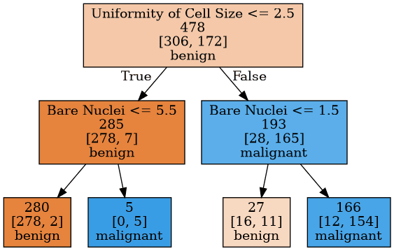
Figure 1: A Simple Decision Tree

In Figure 1, there is a decision tree built based on Wisconsin Breast Cancer dataset from UCI Machine Learning Repository. At each node, there is a condition that splits the data, for example 'Uniformity of Cell Size $\leq$ 2.5' or 'Bare Nuclei $\leq$ 1.5'. Nodes at the bottom are leaves that's classifying the tumors that reaches them as benign or malignant.

We see that, at the left most leaf, there are $278+2=280$ members (tumor records). These are from training data that the tree is built from. The model classified this leaf as benign because the majority class was benign. Every new observation that falls into that leaf will be classified as benign. 280 members of the training data reached this leaf. 278 of them were benign and 2 of them were malignant. So, it's logical to label this leaf as benign because it's the majority class. On the other hand, second leaf from the right does not look good. There are 16 benign and 11 malignant tumors that fell into that leaf and because we label the leaf as whatever the majority class is, it's been labeled as benign. But the frequencies of benign and malignant are very close. The node is non-homogeneous. Maybe it needed further splits.

Another thing that we might have been asked is, in the root node, for example, how did we decide to split the node by the condition 'Uniformity of Cell Size $\leq$ 2.5'? How did we determine that 2.5 boundary? There must be some mechanism that help us decide the 'best split' in a specific node.

So, there should be two important aspects to consider in tree building process. At each node, we check if it might be a good idea to split that node further and find what is the best possible split criterion that creates homogeneous (pure) child nodes.

How can we measure the impurity of a node? One possible measurement is cross-entropy, which is defined as: $$ \sum \limits_{i=1}^{K} - p_i \log p_i \tag{1} $$

where K is the number of classes, 2 for the tumor case. $p_i$ is the proportion of class $i$ in the node and defined as: $$p_i = \frac{N_i}{N}$$ where $N_i$ is the number of members that belong to class $i$ in the node and $N$ is total members in the node.

Another impurity function is gini coefficient: $$1 - \sum \limits_{i=1}^{K} p_i^2 \tag{2}$$

So, we calculate the impurity of a node by an impurity measurement function. We want to create pure leaf nodes. To do that, we must select at each splitting stage, the split that reduces the impurity most. We need to calculate the impurity after the split.

Suppose that a splitting criterion, $C_i$, splits a node into $n$ nodes. Choosing the cross-entropy as our impurity measure, impurity after the split is defined as: $$ \displaystyle{ \mathrm{I'} = - \sum \limits_{j=1}^{n} \frac{N_j}{N} \sum \limits_{i=1}^{K} p_{ij} \log p_{ij} } \tag{3} $$

We choose the split, $C$, that reduces the cross-entropy most. In other words, at a node m, we're looking for a $C$ that maximizes the cross-entropy decrease, which is defined as: $$ \displaystyle{ D(m) =\mathrm{ I_m }- \mathrm{I^{'}_m} } \tag{4} $$

where $\mathrm{I_m}$ is from $(1)$ and $\mathrm{I'_m}$ is from $(3)$. They are calculated based on the node m.

With these fundamental ideas in our mind, let us further explore decision trees by looking at the tree building process.

How to Build a Decision Tree

There are different algorithms for decision tree building. But their core ideas are same. They only differ in data type treatment, tree structure and some additional heuristics.

Suppose that we have $n$ explanatory variables. If an explanatory variable $x_i$ is categorical and has $M$ distinct values, there are $2^{M-1}-1$ different splits. An example split would be $C(m) = 1(x_i = m)$ where $m$ is a possible value that $x_i$ can have. $1(.)$ is the indicator function that returns 0 or 1 based on the boolean expression that it receives as argument. So, the example split, splits the node into two different sets. Therefore, it creates a two different node. If $x_i$ is a numerical (continuous) variable, it can have infinite number of values. But because we can not search for every possible numerical value, we look for the boundary values in our training data. So, that leaves us out with $M-1$ possible splits. For example, suppose that we have a training set that contains $N$ records and suppose that we have an explanatory variable $x_i$ and has values $S_i = { x_i^{(j)}}_{j=1}^{N}$ such that $S_i$ is sorted. We check the possible splits, $C_i(m) = 1(x_i < m)$ where $\displaystyle{m=\frac{ x_i^{(j)} + x_i^{(j+1)} }{2}}, j=0,1,2,...,m-1$. This form of split, again, splits a set into two distinct sets. These are the basic splitting criteria that we will use.

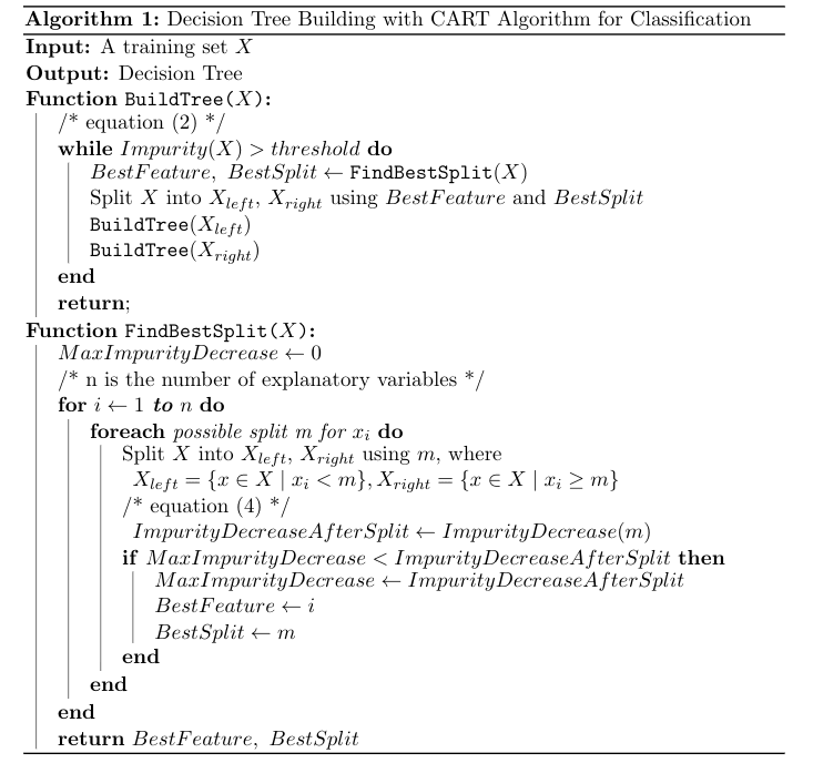
Let us start with the simplest one, the CART algorithm. CART uses the gini index as splitting criterion. Also, CART treats every variable as numerical. So, it always look for split in the form $C(m) = 1(x<m)$. Hence, it always does binary splitting. So, it creates binary trees. Starting from a single node, for each variable, it finds the best split $C_i(m)$, and selects the best split among these variables. In another words, it selects the split that maximizes the impurity decrease from $(2)$. And it recursively repeats this process until there is no decrease in the impurity or the impurity of the current node is less than some threshold value.

Basic CART algorithm is given above. Only one stopping criterion is given in the algorithm. It stops when the current node's impurity is less than or equal to some user-defined threshold. But there are other stopping criteria as well. For example, enforcing a maximum depth to the tree. When the tree reaches to a specified maximum depth, the algorithm stops. Or specifying the minimum members at a node to make it a leaf. When a node has less than or equal number of members inside it, the algorithm stops. These stopping criteria prevents the tree from growing too large. Consequently, prevents overfitting. These criteria often referred as pre-pruning, meaning that pruning the tree while building it. There are also post-pruning techniques which prunes the free after it is grown. We won't discuss post-pruning in this article.

Ensemble Learning

Basic idea behind the ensemble learning is combining multiple base learners to create a powerful model that has higher performance than each individual learner's performance. There are two popular methods for ensemble learning: bagging and boosting. Bagging works by training multiple learners on a sample drawn from the training set. And in prediction time, it takes the average of each learner's prediction (for regression) or it take the majority vote (for classification). Boosting has a different approach. It starts with a 'weak learner' that performs slightly better than random guessing. And it iteratively adds new weak learners to the model to fix the errors that the previous learners made.

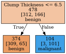
Figure 2: A Decision Stump

Decision trees are often used as base learners in ensemble methods. In bagging, multiple large trees with high variance are trained on different samples of the training set in order to create a robust model that has low variance. In boosting, decision stumps or small trees are often used as high biased learners. A decision stump is a decision tree which goes only one level deep. It does only one decision. In Figure 2, there is an example decision stump built from wisconsin breast cancer data set. It only uses the feature 'Clump Thickness' and makes a single split.

Bagging

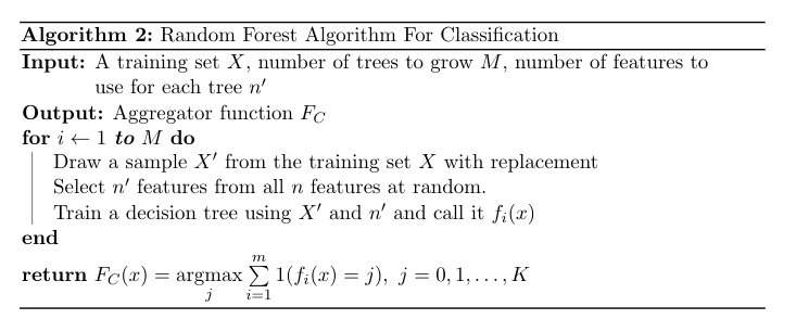
The term bagging stands for 'bootstrap aggregation'. Let's define bootstrapping and aggregating. Bootstrapping is any method that uses random sampling with replacement, which means some sample may have repeated observations. Aggregating means combining the results taken from the different samples.. In the regression case, 'combining' means is taking the average of the results (5). In classification, it means taking the majority vote (6). It turns out that taking bunch of samples with replacement, training some models on them and aggregating the results has a variance reducing effect. Therefore, by bagging, a model with low variance model can be obtained by using high variance models. $$F_R(x) = \frac{1}{m} \sum \limits_{i=1}^{m} f_i(x) \tag{5}$$

$$F_C(x) = \underset{j}{\operatorname{argmax}} \sum \limits_{i=1}^{m} 1(f_i(x) = j), \ j = 0, 1, \dots, K \tag{6}$$

m is the number of trained models.

Random Forest

Random Forest is an ensemble learning algorithm that leverages bagging and decision trees. Decision trees are great choice for ensemble methods because they usually have high variance. Multiple decision trees can be used together to both reduce their individual variances and make use of their power in capturing non-linear relationships in the data.

Besides using decision trees, Random Forest does more one thing to create less correlated tree to reach more predictive performance. If some features in our data set are more correlated with our target features, then every decision trees will use those features to make prediction and therefore, all the trees will be correlated with one another. So, we would end up with trees that are mostly identical to another and our overall model would have low performance. What Random Forest does to prevent this problem is this: For each tree, it uses only a portion of the features in the data set rather using all features. Number of trees and number of features to uses at each tree building process are hyperparameters to tune.

Resources

In this section, I'll give the resources I used while preparing this article that consists of three part.

You can download the Wisconsin Breast Cancer Data Set from here: https://archive.ics.uci.edu/ml/datasets/Breast+Cancer+Wisconsin+(Diagnostic).

Ethem Alpaydın's Introduction to Machine Learning book has a great Decision Tree chapter that gives a solid introduction. Stanford University's CS229 course has useful material in various topics including Decision Trees, Random Forest, Boosting, etc.

A couple of detailed material about CART can be found from these links: 1 2

Elements Of Statistical Learning book by Trevor Hastie, Robert Tibshirani, Jerome H. Friedman is a great book that covers lots of topics in Machine Learning. It has separate dedicated chapters about the topics covered in this article and it gives clear, detailed explanations about these topics.

Jerome H. Friedman's Greedy Function Approximation: Gradient Boosting Machine paper gives a thorough description of Gradient Boosting algorithm and derives several algorithms using Gradient Boosting.

XGBoost: A Scalable Tree Boosting System paper by Tianqi Chen and Carlos Guestrin describes the XGBoost framework. Interested readers are encouraged to read it if they want to learn about what optimizations XGBoost does more deeply.

Python Implementation

You can check the Python implementations of the algorithms that are covered in this post and the two of the upcoming posts in this repo: Tree Based Methods. You can also obtain the pdf version of these 3 posts in the repo.